


back to homepage
Random Boolean Networks are generalized CA's. They can be used to model (certain aspects of real) neural networks and also gene regulation in organisms, because they are composed of many more or less randomly connected elements, which interact with each other according to many different rules.
Random Boolean Networks (RBN) are accordingly discrete dynamical cellular systems, but with exclusively TWO-VALUED variables -- so called Boolean Variables [In CA's, on the contrary, also more-than-two-valued variables are allowed, say, 5-valued variables (i.e. each cell can be in one out of five possible cell states]. In RBN such a boolean variable assigns one out of two possible values to a cell state. Conventionally we accordingly describe a cell of a boolean network as either finding itself in state 0 or in state 1. This property is in accordance with the (idealized) situation in neurons -- they either fire, or do not -- and in genes -- they either are active or are not.
So while CA's usually serve as models of physical (self-organizing) processes, RBN's will normally be used to model some biological functions, especially by reason of their generalized nature, that will be expounded below.

Figure 1. Some typical (local) neighborhoods for (different) CA's.
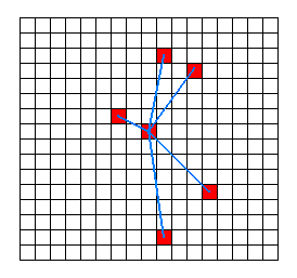
Figure 2. A typical (non-local) neighborhood for an RBN.
Also the size of such a neighborhood does not need to be the same for every neighborhood. So every cell can be differently, and arbitrarily wired to a set of other cells anywhere in the grid, forming its non-local neighborhood. In this way a complex network of (wired) cells can be formed.
[Recall that an attractor of a dynamical system is either a certain system state in which the system finally settles itself (steady state), or a set of system states through which the system finally cycles and keeps on cycling, while revisiting those states again and again (periodic attractor) [NOTE 1a].
A series of successive system states that leads to a certain attractor is called a trajectory. Often many (different) trajectories lead to the same attractor. Such an attractor, together with all the trajectories leading to that attractor, is called the basin of attraction (attraction basin) with respect to that particular attractor (See Figure 3).
The Basin-of-Attraction Field (Attraction Basin Field) is the total of all the attraction basins of the system. And this system could be a Random Boolean Network. So the Basin of Attraction Field displays all the possible connections between the system states, i.e. it displays all possible (system) state transitions with respect to the dynamical system in question.]
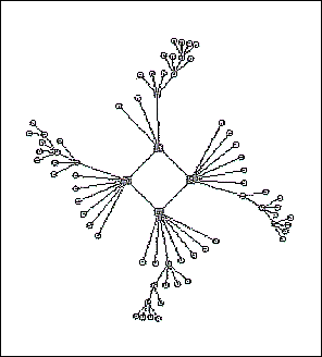
Figure 3. A possible basin of attraction belonging to the Basin of Attraction Field of a Random Boolean Network. Trajectories, starting from initial system states, lead to an Attractor. The Attractor depicted is a 4-cycle, which means that the system, after having reached the attractor, cycles forever through (only) four system states.
In the case of RBN's we will, in contrast with CA's, generally not encounter system states which look each for themselves orderly in a spatial sense. The (root of the) orderliness of the system must be located in factors that are responsible for bringing the system (the network) quickly to a short cycle (attractor), implying that the system eventually resides in a very small region of the State Space of the system (i.e. the space of all possible system states). The cycling activity is now the orderliness of the system.
As has been said, RBN's can be used for the simulation of some biological functions.
Let us, for a better understanding, have a closer look at such a (Random) Boolean System (network).
The system elements (cells) of such a system can -- by definition -- find themselves only in one out of two states : 1 or 0 (ON or OFF, BLACK or WHITE). Cell states are accordingly boolean variables (variables with only two possible values). In Logic we also have to do with such boolean variables : a proposition is either TRUE or FALSE.
Let us investigate a very small and simple Boolean (dynamical) system (Boolean Network) consisting of a one-dimensional row of 19 cells (n = 19). Some cells are in state 0 (OFF), some are in state 1 (ON). This can be interpreted as a start-configuration (initial state) of the system. An example of a start configuration of that system is the following :
1110100001101011111
We shall denote the corresponding cell locations in the one-dimensional grid as follows :
C1 C2 C3 C4 C5 C6 C7 C8 C9 C10 C11 C12 C13 C14 C15 C16 C17 C18 C19
So Cell C1 finds itself in state 1, cell C2 finds itself in state 1, etc.
Such a system can accordingly find itself in one out of 219 (= about 1 million) system states.
Suppose that our system consists of cell neighborhoods with varying size k. Then we can imagine the following configurations :
One or more neighborhoods having k = 3 [i.e. we have one or more cells, each having a neighborhood of three cells. Differently said : one or more cells are each wired to three cells (one of these three cells may, but need not, be the cell itself, in this case the cell is wired to itself and to two other cells)]. In addition to this we could have one or more cells each possessing a neighborhood with k = 4. Each of these cells is thus wired to four cells. Further we could have neighborhoods of other sizes, for example with k = 5, k = 2, k = 9. So to each cell Ci a determined, generally non-local, neighborhood is assigned.
Let us now do that explicitly :
To cell C1 we assign the k = 3 neighborhood C1 C3 C17, and this means that the update of this cell C1 (thus its state at the next point in time t + 1), is dependent on the state-configuration of three cells :
C1           C3           C17

0            0            0
0            0            1
0            1            0
0            1            1
1            0            0
1            0            1
1            1            0
1            1            1
State Transition Rule.
TIME  t                           TIME  t + 1

C1       C3       C17              C1

0        0        0               0
0        0        1               0
0        1        0               0
0        1        1               0
1        0        0               0
1        0        1               0
1        1        0               0
1        1        1               1
The Rule (right column) for cell C1 is thus : 00000001.
This means that if the neighborhood configuration of cell C1 at time t turned out to be 000, then cell C1 acquires the value 0 at the time t + 1 . If the neighborhood configuration turned out to be 001, then the value would also become 0. Et cetera. So the Rule consists of eight if ...... then expressions.
C3    C10

0     0
0     1
1     0
1     1
Suppose that we assign to cell C2 the following Rule (Boolean function, State Transition Rule) :
TIME t          TIME t+1
C3    C10         C2

0     0          0
0     1          1
1     0          1
1     1          1
So the Rule for cell C2 is : 0111 .
In an analogous fashion we can assign a neighborhood (= wiring) and a Rule to every cell of the system, thus to the remaining cells C3 C4 C5 ... C18 and C19, (whereby the size of the neighborhood and the position of the cells of the neighborhood, and the Rule, may differ from cell to cell).
In this way we have set up a NETWORK, a dynamical network.
When we start to run such a network (Boolean Network) with one or another chosen initial system state, i.e. one or another configuration of 19 ON/OFF cells, then the system will update all its cells [ NOTE 2 ]. When this is done, and we find ourselves now at time t + 1, the process will be repeated and applied to the result (i.e. the result now serves as initial system state), producing a new result to which the process is again applied, etc. etc. (and as such it is a typical example of a recursive dynamical system). When we simulate this on a computer -- because to do this manually is inconvenient, if not impossible -- we get a succession of system states (element configurations) which can be displayed on the computer screen. But because the neighborhoods (and thus the dependency relations) are non-local (meaning that the ' neighborhood ' of a cell will not necessarily consist of its immediate spatial neighbors -- like, by the way, the non-locality in many biological systems), we will generally not encounter any system state having a spatially patterned structure (In one-dimensional systems such patterning is hard to discern anyway, but in two-dimensional Boolean systems (thus with a two-dimensional grid of cells) we also will not generally encounter any spatial patterning). The system states look chaotic or in any case irregular. When we look for ORDER in such systems, it is not morphological order but dynamical order, i.e. orderly behavior, that we should look for. It turns out, however, that behavior is also often not orderly in such systems. All Boolean systems, provided they are finite with respect to their number of elements, do, it is true, always finally end up in a cyclic attractor and then behave orderly (From that point onwards they accordingly remain dwelling in just a tiny corner of state space), but it could take a long time for the system to reach this attractor, in those cases where the system is large. Even if we assume that a systemstate-transition takes no longer than a second, it could take billions of years before the cyclic attractor has been reached (and consequently orderly behavior begins). In fact (i.e. in practical terms) such a system can be considered chaotic and does not show any orderly behavior.
Suppose we have a random boolean network consisting of 100000 cells (system elements) [NOTE 3]. The number of possible ON/OFF configurations is 2100000 and that is about 1030000.
This number (but surely also already the number 235000 [= about 1010000] which corresponds to the number of possible ON/OFF configurations of human genes) defies every imagination [NOTE 4].
Can such a system nevertheless reach orderly behavior within a reasonable time span? Can such a huge system, while moving through this 'space' of 1030000 possible states, quickly reach a short cycle of, say, only 300 system states? And can such a system, starting from another initial system state, swiftly reach another short cycle? In other words can such a huge system nevertheless behave orderly?
Yes it can.
According to KAUFFMAN, 1996, At home in the universe, p. 109, the following applies : With k = 2, and more generally, with canalyzing networks (see below) the median number of state-cycle attractors is only about the square root of the number of system elements n. So if n = 100000 then we have a little more than 300 state-cycle attractors.
So it is possible :
IF we take a Boolean system consisting of 100000 elements, in which we assign at random to every cell a Boolean function, and if we also take care that the wiring is such that the size of the neighborhoods is equal to two (k = 2), but with a random location (of the elements of these neighborhoods) in the network, causing those neighborhoods to be non-local[NOTE 5], THEN this huge Boolean network will quickly settle on a small cycle (a cycle with a relatively short period). From another initial state it settles either on this same cycle, or on another cycle which is also small.
KAUFFMAN, (1996, At home in the universe), who discovered this, calls it
"order for free", which means that the system needs almost not to be 'engineered' (crafted) to make it orderly (so there is no need for a rational Creator).
When the wiring is denser, for instance k = 3 (neighborhoods consisting of 3 elements), k = 4, k = 5, then orderly behavior can also emerge provided a large percentage of the rules (Boolean functions, State Transition Rules), assigned to the diverse cells (system elements), is 'canalyzing'. This means that the value which the cell must acquire at its updating should be insensitive with respect to many of the possible neighborhood configurations (value configurations in each neighborhood belonging to a cell to which such a (canalyzing) rule is assigned), for example the Rule :
Neighbor configuration       Output (= Rule s.str.)
(= input)

000                          0
001                          1
010                          0
011                          1
100                          0
101                          1
110                          0
111                          1

TIME t                       TIME t + 1
This Rule accordingly dictates, that IF the third member of the encountered neighborhood is 1, THEN the value of the cell being updated becomes 1, independent of the values of the remaining cells of the neighborhood. If a large percentage of the Rules is in this way canalyzing, then the huge Boolean Network will behave orderly, i.e. it will quickly settle on a small cycle. And from another initial system state it could settle on another small cycle (or maybe on the same cycle). Canalyzing functions, by the way, are easily generated in reality -- i.e. easily from a molecular point of view.
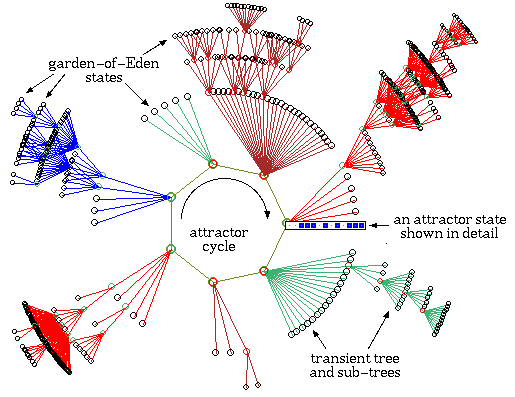
A single Attractor-basin of a Random Boolean Network. The Network consists of 13 cells (system elements (n = 13)), and every neighborhood has a size of 3 cells (i.e. every cell is wired to three cells somewhere in the cel-grid (k = 3)). The complete Basin of Attraction Field is pictured directly below.
( From the Iternet DDLab-gallery of Andrew Wuensche )
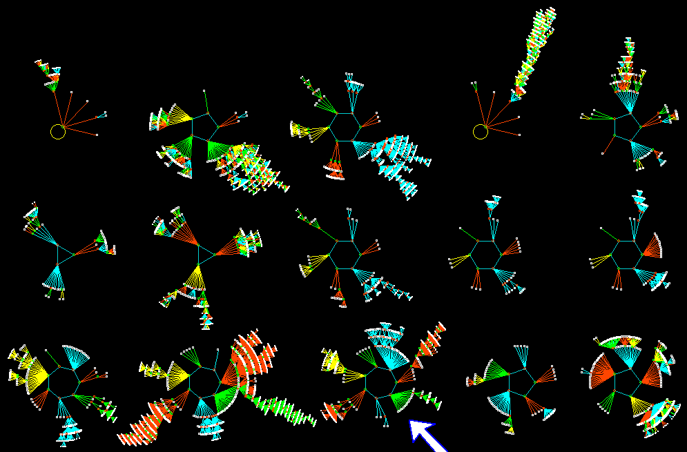
An Attractor-basin Field of a Random Boolean Network. n = 13, k = 3.
( From the Iternet DDLab-gallery of Andrew Wuensche )